COBRA Field Measurements
The Measurement Campaign
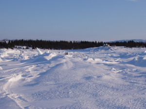
The measurement campaign to address the COBRA objectives took place at Kuujjuarapik, during spring of 2008. The measurements made were wide ranging, and were based at the Laval University Centre d’Etudes Nordique, Kuujjuarapik research station and at a remote site a few kilometres outside the town powered by a generator, including a small ice camp a few hundred metres off the coast on the sea ice. The remote site where most of the measurements were made was immediately on the coast, with the measurement containers approximately fifty metres away from the level sea ice surface and about 6m above it. In the prevailing wind directions air arrives at the site after passing over the Hudson bay, with the last 2-3Km consisting of unbroken sea ice, but with open leads beyond that. There were no local pollution sources in these directions, with the exception of a small amount of Skidoo traffic during the day time from locals travelling out on to the ice. A full list of the measurements made by the various groups participating in the project is contained in the table here. The Manchester measurements will be described in more detail on this page.
Aerosol Size Distribution
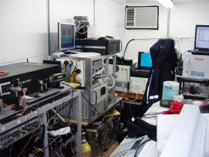
Aerosol size distribution measurements were made using a Differential Mobility Particle Sizer (DMPS), and a GRIMM 1.108 dust monitor. The DMPS classifies particles according to electrical mobility in a differential mobility analyser and counts particles of given mobility using a condensation particle counter. The Manchester DMPS uses two such DMA’s and CPC of different specifications to measure aerosol size distributions from 3.5 – 800nm, with a complete scan taking ten minutes. The GRIMM is an optical particle counter, sizing particles based on laser scattering, it has a size range of 0.3 – 20µm and produces a distribution every six seconds. These instruments were located in one of the sea containers placed on the coast, with aerosol being sampled down a 10mm internal diameter turbulent inlet at 35 lpm from a height of 4m above the ground, which taking into account the height of the shore line gives a height of approx 10m above the sea ice surface. This inlet was fitted with a sharp cut 4um cyclone, to prevent large particles entering the instruments, thus restricting the effective measurement size range to 3.5nm to 4µm. Close to the instruments, the main flow was decelerated allowing it to become laminar and the 3.5 lpm flow required for the instruments was sub-sampled isokinetically from the centre of the main flow. Transmission efficiency through this inlet has been characterised using theoretical calculations for diffusional, inertial and gravitational losses, thus allowing measured size distributions to be corrected for inlet losses. Although for this experiment aerosol were not actively dried, the temperature difference between the interior of the container and the outside air (typically at least 35 deg C) meant that aerosol were sampled dry.
Flux Measurements
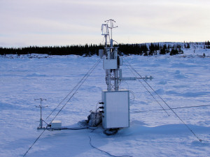
Flux measurements were made at an ice camp approximately 300 metres away from the main site. Two height 20Hz turbulence measurements were made using 3d sonic anemometers mounted on a small mast secured on the sea ice, with measurement volumes at heights of 0.5 and 2.5m. These turbulence measurements allowed eddy covariance measurements of latent and sensible heat, ozone, total and ultra-fine aerosol fluxes. With the exception of sensible heat which was measured at both heights, these parameters were measured at 2.5m above the ice surface. In order to make these measurements additional fast response sensors were deployed on the mast.
To calculate the latent heat flux a Campbell Scientific Krypton Hygrometer was used to measure rapid fluctuations in water vapour concentration. This instrument uses UV absorption to measure these rapid fluctuations, but does not give a reliable absolute concentration, so the data from the krypton hygrometer is coupled with an absolute measurement from a Rotronic T+RH sensor.
Ozone fluxes were measured using a Guston chemiluminescent fast response sensor, which measures rapid fluctuations in ozone concentration, but not absolute concentration as the response of the instrument changes with the age of the target disk. Thus data from the Guston is coupled with an absolute measurement from a 2B ozone analyser also mounted on the mast. The Guston is also sensitive to water vapour, so the water vapour measurements are used to correct for this.
Particle fluxes were measured using two TSI condensation particle counters, a model 3776 which has a lower cut of 3nm and a 3010 which has a lower cut of 10nm. The total particle flux is simply calculated from the fluctuations in the 3776 concentration, while the ultra-fine flux is calculated from fluctuations in the difference between the two concentrations. These particle counters were mounted in a temperature controlled box fitted to the lower part of the mast, and sampled from a 10lpm turbulent inlet line bringing air from close to the sonic anemometer measurement volume. This inlet line was fitted with a miniature impactor with a 2µm cut to prevent large particles entering the instruments. The instrument flow was split from the bypass flow close to the inlet of the instruments using an isokinetic flow splitter. Theoretical calculations of inlet transmission efficiency are used to correct the measured particle concentrations and fluxes for inlet line losses.
In addition to the eddy covariance flux measurements, two height (0 and 1.8m) measurements of aerosol size distribution (0.3 – 20µm) were made with GRIMM optical particle counters. These were mounted on the mast in heated boxes with very short inlets, and so able to measure over their full size range. While these instruments are not fast enough for making eddy covariance flux measurements at these heights, the two height measurement allows for the calculation of fluxes using the gradient method.
Finally long and shortwave net radiation was also measured at the mast using a Kipp and Zonnen net radiometer.
All the data from the instruments on the mast was transmitted back to the container using a wireless Ethernet bridge, and monitored and logged on a computer there. This was especially useful as operating a computer out on the ice was not a very easy or pleasant process.
Chamber Measurements
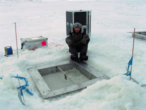
Dynamic flux chambers were deployed close to the ice camp to measure emissions from open leads, newly formed sea ice and frost flower structures. Three sites for such chambers were selected within one hundred metres of the main ice camp measurement location. At each site a 1m square hole – an artificial lead – was dug through the ice, which turned out to be a little over 1m thick. The base portion of a chamber was fitted to each hole and allowed to freeze into place creating an airtight seal with the ice. Between chamber experiments the hole within the chamber base was cleared of ice twice daily to prevent too great a build up of ice. When a chamber experiment was to be carried out, a Teflon film covered chamber lid was fitted onto the base, enclosing a volume of approximately 100l. The enclosed volume was stirred to prevent a vertical concentration gradient developing. Multiple chambers sites allowed measurements to be made over ice surfaces at different stages of development, and allowed surfaces at each location to be re-exposed to the atmosphere to minimise microclimate induced changes which may occur within the chambers.
Concentrations of I2, halocarbons and aerosol particles were sampled from the chamber at regular intervals as the ice and frost flowers developed. A temperature profile within the water/ice and the air immediately above it was measured continuously throughout the experiment, and the development of the ice and frost flowers was recorded with a web cam. I2 and halocarbons were measured using tube trapping techniques for later analysis. I2 was trapped on starch coated ambered glass tubes, two of which were taken per chamber run. These were stored and transported back to the UK for analysis. Halocarbons were trapped in commercially available three adsorbent filled stainless steel tubes, several of which were taken per chamber run. These tube sample were thermally desorbed and analysed on a Gas Chromatogram at the research station. I2 and Halocarbon sampling and analysis was carried out by the York group. Aerosol number concentration in the chamber was monitored during the experiment using a TSI 3025 condensation particle counter, which outputs total aerosol number greater than 3.5nm diameter.
It was found that under the correct conditions a frost flower structure would develop typically within 24 hours of an artificial lead being created. It was found that low wind, and protection from direct sunlight (ie cloud cover or darkness), as well as low temperatures provided the ideal conditions for frost flower formation on the artificial leads. It was also observed that frost flower formation took place on similar timescales on an area of ice close to the shore which became flooded due to tidal activity.