Holme Moss PROCLOUD Project - Results
Flow connection and dilution
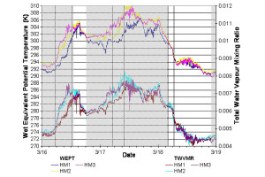
Flow connectivity between sites, when the wind direction was favourable, was analysed by comparing the conserved thermodynamic properties, wet equivalent potential temperature and water vapour mixing ratio of the air mass. These parameters were calculated from temperature and relative humidity at each site measured using Vaisalla sensors. Wet equivalent potential temperature is defined as the temperature an air parcel would have at a pressure of 1013.25 mbar with all water vapour condescend out and the latent heat released used to increase the temperature of the air. Water vapour mixing ratio is simply the concentration of water vapour and is sometimes also referred to as absolute humidity. When in cloud condensed water content must also be included in the conserved quantity.
Figure 1 shows comparisons of wet equivalent potential temperature and water vapour mixing ratio for all three sites, which shows periods with and without connected flow. Generally it was found that for most of the time thermodynamic properties indicated sites HM2 and HM3 to be connected, but HM1 was often disconnected, especially when the wind speed at this site was low. However, in some cases, even when thermodynamically connected, other indicators such as aerosol number and gas phase concentrations showed significant differences between the sites, suggesting that the Manchester plume was being diluted into thermodynamically similar air.
Gas phase data
Gas phase measurements made at both HM1 and HM2 showed evidence of significant anthropogenic influence, with concentrations of NOx rising from a background of 5 ppb to peaks of 45 ppb upwind and 20 ppb at the summit. NOx was observed to exhibit a broad diurnal cycle, which was most evident at HM1, and was strongly anti-correlated with O3. In figure 2 a week of NO2 and O3 data is plotted which clearly shows this diurnal cycle and anti-correlation. This anti-correlation is due to gas phase chemical reactions between O3 and NOx, providing evidence that most of the NOx present was emitted as NO, which is typical of emissions from combustion processes, and has been converted to NO2 by the following reaction:
NO + O3 --> NO2 + O2
Generally, differences between HM1 and HM2 can be explained by the Manchester plume having been diluted as it is transported between the sites. However it was also observed that transport between sites affects NO2 and O3 differently, indicating that gas and aqueous phase chemical processes may also be important in the removal of NO2.
SO2 data from HM1 and HM2 shows no clear diurnal cycle and no evidence of dilution between sites, with concentrations at HM2 often higher than those at HM1. This suggests that SO2 is not originating in the Manchester plume, but from sources upwind of Manchester. Such sources would include the coal fired power station at Fiddler’s Ferry near Warrington, and the large oil refinery at Ellesmere Port, Cheshire. There are also other large industrial sources of SO2 in these areas.
Measured concentrations of H2O2 (which is an important aqueous phase oxidant when dissolved into cloud droplets) at HM1 were low, usually less than 0.5 ppb, and often less than the detection limit of the instrument. Since H2O2 is photochemically produced, large concentrations would not be expected during the winter. NH3 concentrations at both HM1 and HM3 were high, at up to 10 ppb at the start of the project, and very low towards the end. As both these sites were located on agricultural land (sheep and dairy farms), these high concentrations were probably as a result of local emissions and were not thought to be representative of NH3 concentrations throughout the cloud. In the absence of high levels of H2O2, and with relatively high concentrations of SO2 present, NH3 concentrations are very important for cloud processing. Dissolved NH3 regulates the pH of cloud droplets, and under these conditions is a key factor in controlling sulphate production.
Aerosol number
Aerosol number measured at all sites exhibited a diurnal cycle, with a daytime maximum of up to 80,000 cm-3 and a night time minimum of about 5000 cm-3. Concentrations at HM1 were generally higher than those at HM2, often by a factor of 2 or larger, though at other times concentrations at HM2 were equal to or greater than those at HM1.
Aerosol size distributions
DMPS spectra measured at the upwind site are somewhat variable, with the shape of the spectra being very dependant on prevailing pollution conditions. Figure 4 gives examples of spectra at different points in the diurnal cycle in total aerosol number, for 18th March, a day during which connected flow existed between the sites for most of the time. From the figure it can be seen that the distribution is broad throughout the day, but that the peak moves to smaller sizes under more polluted conditions. Under relatively clean conditions during the night there is only one main mode, with a very broad peak between 20 and 100 nm, and in some cases a small ultra-fine mode with a peak at 5 nm. Under more polluted conditions during the day, there is a broad nucleation mode with a peak typically between 10 and 20 nm, and a relatively small accumulation mode with a peak at about 200 nm. Other days show similar spectra under these types of conditions.
Aerosol hygroscopicity and chemical composition
Measurements of aerosol hygroscopic properties throughout the project showed that in most cases an external mixture of aerosol having different hygroscopic properties was present. For the largest particles measured (440 nm) most particles were in the hygroscopic mode, with a growth factor of between 1.8 and 1.9. However, a second hydrophobic mode was present for 70% of measurements, had an average growth factor of 1.04, and accounted for 26% of particles. At smaller sizes a much more significant fraction of particles were in the hydrophobic mode. For 35 nm particles the hygroscopic mode had a growth factor of between 1.36 and 1.55. Additional modes were present for 96% of measurements, and contained between 54 and 86% of particles. For 90% of measurements the additional mode was hydrophobic, with a growth factor of 1.09, and for 6% of measurements, in addition to the hydrophobic mode, a less hygroscopic mode with a growth factor of 1.33 was present accounting for 56% of particles. These measurements suggest that the small aerosol which are present under heavily polluted conditions have a very small soluble fraction, and are mostly composed of hydrocarbons and other by-products of combustion.
Berner impactor measurements of the aerosol soluble fraction for aerosol larger than 100 nm showed that this consisted of mostly ammonium sulphate and ammonium nitrate, with smaller amounts of sodium chloride. Significant amounts of potassium, magnesium, and calcium were also present in some cases, with these species accounting for up to 45% of aerosol mass in the larger particles, especially when total aerosol loading was low. The presence of these species suggests that some aerosol may have originated through mechanical production from the ground, with dust from cement works being a strong source of this type of aerosol. Figure 5 shows average Berner impactor data for background polluted conditions, and very polluted conditions. Although not shown by this figure, most of the additional mass is added to the 0.316, 0.681 and 1.47 µm categories, with mass in these categories typically increased by a factor of between 2 and 4. Approximately 95% of this additional mass is due to increased loadings of ammonium (34%), nitrate (32%) and sulphate (29%).
Cloud microphysics
Figure 6 shows a comparison between FSSP droplet number, and ASASP-X aerosol number from HM3, downwind aerosol data has been used to avoid problems of dilution between the upwind and summit sites. This figure shows a significant sub-linear relationship between droplet and aerosol number, with droplet number only rarely greater than 600 cm-3 regardless of aerosol number. Only with low aerosol number is there any relationship between aerosol and droplet number.
Evidence of cloud processing of aerosol
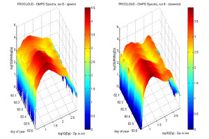
Dilution of the air from the upwind site as it passes over the hill complicates the issue of identifying effects of passage through cloud. For all cloud runs where connected flow existed between all three sites, aerosol spectra show some evidence of cloud processing, an example of which is shown in figure 7. This behaviour is not seen in spectra for other periods of time when cloud is not present.